Mostrando entradas con la etiqueta geometría. Mostrar todas las entradas

domingo, 7 de septiembre de 2014

Neurons in human skin perform advanced calculations

[2014-09-01] Neurons in human skin perform advanced calculations, previously believed that only the brain could perform. This is according to a study from Umeå University in Sweden published in the journal Nature Neuroscience.


A fundamental characteristic of neurons that extend into the skin and record touch, so-called first-order neurons in the tactile system, is that they branch in the skin so that each neuron reports touch from many highly-sensitive zones on the skin.

According to researchers at the Department of Integrative Medical Biology, IMB, Umeå University, this branching allows first-order tactile neurons not only to send signals to the brain that something has touched the skin, but also process geometric data about the object touching the skin.

- Our work has shown that two types of first-order tactile neurons that supply the sensitive skin at our fingertips not only signal information about when and how intensely an object is touched, but also information about the touched object's shape, says Andrew Pruszynski, who is one of the researchers behind the study.

The study also shows that the sensitivity of individual neurons to the shape of an object depends on the layout of the neuron’s highly-sensitive zones in the skin.

- Perhaps the most surprising result of our study is that these peripheral neurons, which are engaged when a fingertip examines an object, perform the same type of calculations done by neurons in the cerebral cortex. Somewhat simplified, it means that our touch experiences are already processed by neurons in the skin before they reach the brain for further processing, says Andrew Pruszynski.

For more information about the study, please contact Andrew Pruszynski, post doc at the Department of Integrative Medical Biology, IMB, Umeå University. He is English-speaking and can be reached at: 
Phone: +46 90 786 51 09; Mobile: +46 70 610 80 96


ORIGINAL: Umeå University

lunes, 17 de marzo de 2014

The 17 Equations That Changed The Course Of History

Mathematics is all around us, and it has shaped our understanding of the world in countless ways.

In 2013, mathematician and science author Ian Stewart published a book on 17 Equations That Changed The World. We recently came across this convenient table on Dr. Paul Coxon’s twitter account by mathematics tutor and blogger Larry Phillips that summarizes the equations. (Our explanation of each is below):
 Stewart 17 equations table
Here is a little bit more about these wonderful equations that have shaped mathematics and human history:
Pythagorean theorem chalkboard
1) The Pythagorean Theorem: This theorem is foundational to our understanding of geometry. It describes the relationship between the sides of a right triangle on a flat plane: square the lengths of the short sides, a and b, add those together, and you get the square of the length of the long side, c.
This relationship, in some ways, actually distinguishes our normal, flat, Euclidean geometry from curved, non-Euclidean geometry. For example, a right triangle drawn on the surface of a sphere need not follow the Pythagorean theorem.

2) Logarithms: Logarithms are the inverses, or opposites, of exponential functions. A logarithm for a particular base tells you what power you need to raise that base to to get a number. For example, the base 10 logarithm of 1 is log(1) = 0, since 1 = 100; log(10) = 1, since 10 = 101; and log(100) = 2, since 100 = 102.
The equation in the graphic, log(ab) = log(a) + log(b), shows one of the most useful applications of logarithms: they turn multiplication into addition.
Until the development of the digital computer, this was the most common way to quickly multiply together large numbers, greatly speeding up calculations in physics, astronomy, and engineering.

3) Calculus: The formula given here is the definition of the derivative in calculus. The derivative measures the rate at which a quantity is changing. For example, we can think of velocity, or speed, as being the derivative of position — if you are walking at 3 miles per hour, then every hour, you have changed your position by 3 miles.
Naturally, much of science is interested in understanding how things change, and the derivative and the integral — the other foundation of calculus — sit at the heart of how mathematicians and scientists understand change.

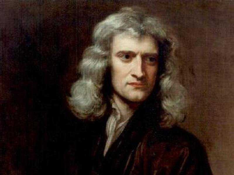
 Isaac Newton
Isaac Newton
4) Law of Gravity: Newton’s law of gravitation describes the force of gravity between two objects, F, in terms of a universal constant, G, the masses of the two objects, m1 and m2, and the distance between the objects, r. Newton’s law is a remarkable piece of scientific history — it explains, almost perfectly, why the planets move in the way they do. Also remarkable is its universal nature — this is not just how gravity works on Earth, or in our solar system, but anywhere in the universe.
Newton’s gravity held up very well for two hundred years, and it was not until Einstein’s theory of general relativity that it would be replaced.

5) The square root of -1: Mathematicians have always been expanding the idea of what numbers actually are, going from natural numbers, to negative numbers, to fractions, to the real numbers. The square root of -1, usually written i, completes this process, giving rise to the complex numbers.
Mathematically, the complex numbers are supremely elegant. Algebra works perfectly the way we want it to — any equation has a complex number solution, a situation that is not true for the real numbers : x2 + 4 = 0 has no real number solution, but it does have a complex solution: the square root of -2. Calculus can be extended to the complex numbers, and by doing so, we find some amazing symmetries and properties of these numbers. Those properties make the complex numbers essential in electronics and signal processing.
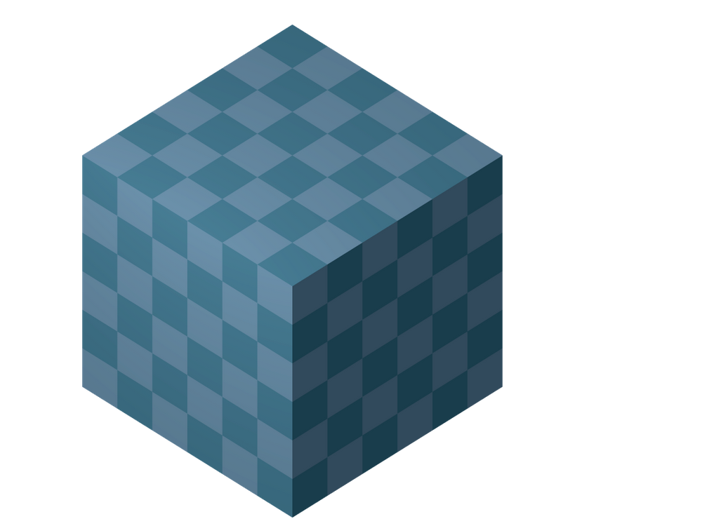
 CubeA cube.
6) Euler’s Polyhedra Formula: Polyhedra are the three-dimensional versions of polygons, like the cube to the right. The corners of a polyhedron are called its vertices, the lines connecting the vertices are its edges, and the polygons covering it are its faces.
A cube has 8 vertices, 12 edges, and 6 faces. If I add the vertices and faces together, and subtract the edges, I get 8 + 6 – 12 = 2.

Euler’s formula states that, as long as your polyhedron is somewhat well behaved, if you add the vertices and faces together, and subtract the edges, you will always get 2. This will be true whether your polyhedron has 4, 8, 12, 20, or any number of faces.
Euler’s observation was one of the first examples of what is now called a topological invariant — some number or property shared by a class of shapes that are similar to each other. The entire class of “well-behaved” polyhedra will have V + F – E = 2. This observation, along with with Euler’s solution to the Bridges of Konigsburg problem, paved the way to the development of topology, a branch of maths essential to modern physics.
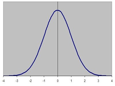
 Bell curve
The normal distribution.
7) Normal distribution: The normal probability distribution, which has the familiar bell curve graph to the left, is ubiquitous in statistics.
The normal curve is used in physics, biology, and the social sciences to model various properties. One of the reasons the normal curve shows up so often is that it describes the behaviour of large groups of independent processes.

8) Wave Equation: This is a differential equation, or an equation that describes how a property is changing through time in terms of that property’s derivative, as above. The wave equation describes the behaviour of waves — a vibrating guitar string, ripples in a pond after a stone is thrown, or light coming out of an incandescent bulb. The wave equation was an early differential equation, and the techniques developed to solve the equation opened the door to understanding other differential equations as well.

9) Fourier Transform: The Fourier transform is essential to understanding more complex wave structures, like human speech. Given a complicated, messy wave function like a recording of a person talking, the Fourier transform allows us to break the messy function into a combination of a number of simple waves, greatly simplifying analysis.

The Fourier transform is at the heart of modern signal processing and analysis, and data compression.

10) Navier-Stokes Equations: Like the wave equation, this is a differential equation. The Navier-Stokes equations describes the behaviour of flowing fluids — water moving through a pipe, air flow over an aeroplane wing, or smoke rising from a cigarette. While we have approximate solutions of the Navier-Stokes equations that allow computers to simulate fluid motion fairly well, it is still an open question (with a million dollar prize) whether it is possible to construct mathematically exact solutions to the equations.

11) Maxwell’s Equations: This set of four differential equations describes the behaviour of and relationship between electricity (E) and magnetism (H).

Maxwell’s equations are to classical electromagnetism as Newton’s laws of motion and law of universal gravitation are to classical mechanics — they are the foundation of our explanation of how electromagnetism works on a day to day scale. As we will see, however, modern physics relies on a quantum mechanical explanation of electromagnetism, and it is now clear that these elegant equations are just an approximation that works well on human scales.

12) Second Law of Thermodynamics: This states that, in a closed system, entropy (S) is always steady or increasing. Thermodynamic entropy is, roughly speaking, a measure of how disordered a system is. A system that starts out in an ordered, uneven state — say, a hot region next to a cold region — will always tend to even out, with heat flowing from the hot area to the cold area until evenly distributed.

The second law of thermodynamics is one of the few cases in physics where time matters in this way. Most physical processes are reversible — we can run the equations backwards without messing things up. The second law, however, only runs in this direction. If we put an ice cube in a cup of hot coffee, we always see the ice cube melt, and never see the coffee freeze.

 AP050124019477
Albert Einstein

13) Relativity: Einstein radically altered the course of physics with his theories of special and general relativity. The classic equation E = mc2 states that matter and energy are equivalent to each other. Special relativity brought in ideas like the speed of light being a universal speed limit and the passage of time being different for people moving at different speeds.
General relativity describes gravity as a curving and folding of space and time themselves, and was the first major change to our understanding of gravity since Newton’s law. General relativity is essential to our understanding of the origins, structure, and ultimate fate of the universe.

14) Schrodinger’s Equation: This is the main equation in quantum mechanics. As general relativity explains our universe at its largest scales, this equation governs the behaviour of atoms and subatomic particles.
Modern quantum mechanics and general relativity are the two most successful scientific theories in history — all of the experimental observations we have made to date are entirely consistent with their predictions. Quantum mechanics is also necessary for most modern technology — nuclear power, semiconductor-based computers, and lasers are all built around quantum phenomena.

15) Information Theory: The equation given here is for Shannon information entropy. As with the thermodynamic entropy given above, this is a measure of disorder. In this case, it measures the information content of a message — a book, a JPEG picture sent on the internet, or anything that can be represented symbolically. The Shannon entropy of a message represents a lower bound on how much that message can be compressed without losing some of its content.
Shannon’s entropy measure launched the mathematical study of information, and his results are central to how we communicate over networks today.

16) Chaos Theory: This equation is May’s logistic map. It describes a process evolving through time — xt+1, the level of some quantity x in the next time period — is given by the formula on the right, and it depends on xt, the level of x right now. k is a chosen constant. For certain values of k, the map shows chaotic behaviour: if we start at some particular initial value of x, the process will evolve one way, but if we start at another initial value, even one very very close to the first value, the process will evolve a completely different way.

We see chaotic behaviour — behaviour sensitive to initial conditions — like this in many areas. Weather is a classic example — a small change in atmospheric conditions on one day can lead to completely different weather systems a few days later, most commonly captured in the idea of a butterfly flapping its wings on one continent causing a hurricane on another continent.

17) Black-Scholes Equation: Another differential equation, Black-Scholes describes how finance experts and traders find prices for derivatives. Derivatives — financial products based on some underlying asset, like a stock — are a major part of the modern financial system.
The Black-Scholes equation allows financial professionals to calculate the value of these financial products, based on the properties of the derivative and the underlying asset.
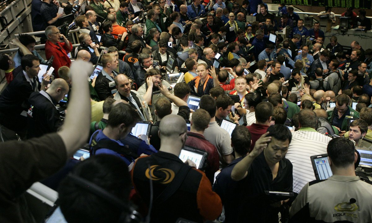
 Cboe stock options traderHere are some traders in the S&P 500 options pit at the Chicago Board Options Exchange. You won’t find a single person here that hasn’t heard about the Black-Scholes equation.


ORIGINAL: Business Insider
Andy Kiersz
Mar 13 2014

lunes, 23 de septiembre de 2013

A Jewel at the Heart of Quantum Physics

By: Natalie Wolchover
September 17, 2013

Artist’s rendering of the amplituhedron, a newly discovered mathematical object resembling a multifaceted jewel in higher dimensions. Encoded in its volume are the most basic features of reality that can be calculated — the probabilities of outcomes of particle interactions. . Illustration by Andy Gilmore
Physicists have discovered a jewel-like geometric object that dramatically simplifies calculations of particle interactions and challenges the notion that space and time are fundamental components of reality.

“This is completely new and very much simpler than anything that has been done before,” said Andrew Hodges, a mathematical physicist at Oxford University who has been following the work.

The revelation that particle interactions, the most basic events in nature, may be consequences of geometry significantly advances a decades-long effort to reformulate quantum field theory, the body of laws describing elementary particles and their interactions. Interactions that were previously calculated with mathematical formulas thousands of terms long can now be described by computing the volume of the corresponding jewel-like “amplituhedron,” which yields an equivalent one-term expression.

“The degree of efficiency is mind-boggling,” said Jacob Bourjaily, a theoretical physicist at Harvard University and one of the researchers who developed the new idea. “You can easily do, on paper, computations that were infeasible even with a computer before.”

The new geometric version of quantum field theory could also facilitate the search for a theory of quantum gravity that would seamlessly connect the large- and small-scale pictures of the universe. Attempts thus far to incorporate gravity into the laws of physics at the quantum scale have run up against nonsensical infinities and deep paradoxes. The amplituhedron, or a similar geometric object, could help by removing two deeply rooted principles of physics: locality and unitarity.

“Both are hard-wired in the usual way we think about things,” said Nima Arkani-Hamed, a professor of physics at the Institute for Advanced Study in Princeton, N.J., and the lead author of the new work, which he is presenting in talks and in a forthcoming paper. “Both are suspect.”

Locality is the notion that particles can interact only from adjoining positions in space and time. And unitarity holds that the probabilities of all possible outcomes of a quantum mechanical interaction must add up to one. The concepts are the central pillars of quantum field theory in its original form, but in certain situations involving gravity, both break down, suggesting neither is a fundamental aspect of nature.

In keeping with this idea, the new geometric approach to particle interactions removes locality and unitarity from its starting assumptions. The amplituhedron is not built out of space-time and probabilities; these properties merely arise as consequences of the jewel’s geometry. The usual picture of space and time, and particles moving around in them, is a construct.

“It’s a better formulation that makes you think about everything in a completely different way,” said David Skinner, a theoretical physicist at Cambridge University.

The amplituhedron itself does not describe gravity. But Arkani-Hamed and his collaborators think there might be a related geometric object that does. Its properties would make it clear why particles appear to exist, and why they appear to move in three dimensions of space and to change over time.

Because “we know that ultimately, we need to find a theory that doesn’t have” unitarity and locality, Bourjaily said, “it’s a starting point to ultimately describing a quantum theory of gravity.”

Clunky Machinery

The amplituhedron looks like an intricate, multifaceted jewel in higher dimensions. Encoded in its volume are the most basic features of reality that can be calculated, “scattering amplitudes,” which represent the likelihood that a certain set of particles will turn into certain other particles upon colliding. These numbers are what particle physicists calculate and test to high precision at particle accelerators like the Large Hadron Collider in Switzerland.

United States Postal Service


The iconic 20th century physicist Richard Feynman invented a method for calculating probabilities of particle interactions using depictions of all the different ways an interaction could occur. Examples of “Feynman diagrams” were included on a 2005 postage stamp honoring Feynman.

The 60-year-old method for calculating scattering amplitudes — a major innovation at the time — was pioneered by the Nobel Prize-winning physicist Richard Feynman. He sketched line drawings of all the ways a scattering process could occur and then summed the likelihoods of the different drawings. The simplest Feynman diagrams look like trees: The particles involved in a collision come together like roots, and the particles that result shoot out like branches. More complicated diagrams have loops, where colliding particles turn into unobservable “virtual particles” that interact with each other before branching out as real final products. There are diagrams with one loop, two loops, three loops and so on — increasingly baroque iterations of the scattering process that contribute progressively less to its total amplitude. Virtual particles are never observed in nature, but they were considered mathematically necessary for unitarity — the requirement that probabilities sum to one.

miércoles, 30 de mayo de 2012

Geometry Of The Big Bang

ORIGINAL: Science20
May 28th 2012

The deeper we look into the universe, the deeper we look back in time. When in the night sky you see planets like Jupiter and Saturn, you look about an hour back in time. Look at the stars, and you are looking back in time anywhere from years to several centuries. Bring a binocular to a dark site and you will be able to see galaxies millions of years back in time. Get a decent telescope to the same site and you look even further back. 

However, there is a limit to how deep you can peek. No matter what equipment you bring, and no matter what part of the electromagnetic spectrum you observe, you can't look back more than 13.7 billion years. What do we see when looking at these times long past? A glow. A nearly uniform microwave glow across the full sky. The cooled-down remnant of the fierce flash of light emitted at the dawn of time.

Visualizing The Big Bang
If you accept these words about the big bang radiation at face value, you are probably not giving them enough thought. Just think for a moment about this radiation surrounding us. Does that make sense? How can we be surrounded by radiation from the big bang 13.7 billion years after the fact? Ignite a bomb, or do whatever you need to do to cause a fireball that emits light and matter. No matter how big a fireball you create, the light will fly out faster than the matter. As a result, observers who are part of the explosion and fly out with the ejected matter, will not keep up with the light and soon not see any of it. So how on earth can we be swimming in the light from the explosion that we ourselves are part of?

Ok, you probably know the reply to this objection: the big bang was not an explosion that happened somewhere. It was an explosion that happened everywhere. Knowing this answer, how do you visualize the big bang? As some giant carpet bombing?

Such visualizations don't make much sense. Any carpet bombing analogy leads to an avalanche of more problematic questions. Who or what orchestrated all these bombs and made them ignite at the same time? And how can it be that the radiation from the big bang is uniform across the sky? Uniformity means each individual bomb in this carpet bombing not only ignited simultaneously, but also each bomb must have been an accurate copy of all the others. Who ordered these zillions of copies of the same bomb, and made them ignite at the same time?

Most pop science books when reaching this point will make some remarks about bombs explodingin space while the big bang creates space. This is the moment in the discussion where galaxies get depicted as raisins in expanding bread dough. Yet, such considerations and analogies do not make the uniformity riddle, referred to by cosmologists as the "horizon problem", go away.

At this point your favorite pop science books will probably introduce the concept of cosmic inflation. As this follows the picturing of our universe as rising bread dough, this leaving the reader with a vague notion of a magical multiplication of dough preceding the baking of the cosmic raisin bread.

If all of this is a reliable description of the big bang theory of cosmology, you should not believe a word of this theory. But of course it isn't. Cosmologists don't need any magical bread multiplication. Forget loafs of bread, forget exploding bombs, forget rubber sheets or whatever you were made to believe represents the big bang. Today, I will present you with a much more satisfying visualization. A visualization that captures the main features of the early universe and that also depicts quite accurately the late stage of evolution the universe has entered. This visualization is relativistically correct, it features an accelerating expansion, and it depicts what is without any doubt the most elegant and most beautiful big-bang model ever constructed.

The visualization will shed new light on the horizon problem, and also suggests an answer to the question "what came before the big bang?". An answer that might surprise you and that at the same time might eliminate any aversion to the big bang cosmology that you might carry with you. And best of all: this relativistic visualization does not require any heavy math. All that is needed is some simple geometrical concepts. The secret to enable this feat is to sacrifice two of the spatial dimensions. This gives us a universe with one time and one spatial dimension that can be visualized as a curled up surface in a 3D space-time.

One last word and a bit of a disclaimer before we start. Is the visualization I will present here the true and unique model of our expanding universe? No it isn't. Firstly, it is an idealized model, and secondly when it comes down to the very early stages of the universe we enter terra incognita. The picture I will present lead us right through the moment of the big bang. Yet, what actually happened at the very moment of the big bang no one can tell for sure. Astronomers can look back down to 380,000 years after the big bang. At the LHC we can recreate the conditions of the universe down to much earlier times of about 0.00000000001 seconds after the big bang. Still earlier times are not experimentally accessible to us, as we lack particle accelerators powerful enough to recreate the energies required. Nobody can claim to know what happened at times and energies not accessible to us. However,we do have theories that go down to much earlier times. All these theories are speculative in nature, and that includes the theory on which below visualization is based.

I should stress here that regardless of these disclaimers, below visualization honors Einstein's well-tested general theory of relativity, and at the same time it avoids any singularities that would make the math blow up. As such it provides us with an excellent tool to sharpen our intuition when it comes to issues like the horizon problem.The whole point here is: learn from this visualization and use it to sharpen your thinking about issues surrounding big bang theories, but don't get carried away into thinking that this is the last and final word on what happened at time zero.

Having said this, despite the physics at time zero being unknown to us, the big bang phenomenon in itself is not in any way speculative. The fact that our universe is expanding is as certain as the fact that earth's surface is curved. The picture that will be presented below gives a description of the universe akin to the spherical earth description. It provides us with the most symmetric description of our universe: a 'spherical space-time' model. As space-time distances don't behave like spatial distances, a 'space-time sphere' takes the shape of a hyperbolic geometry that enforces a description of an accelerating"open universe". Sounds enigmatic? Read on and all will be clear in a few minutes.

Beauty Bouncing Back
In 1917, just two years after Einstein published his general relativity theory, the Dutch mathematician and astronomer Willem de Sitter came up with a four-dimensional space-time that fitted Einstein's equations. The way he obtained his solution was remarkable: De Sitter had started from a five-dimensional hyper-space-time in which he 'carved out' a four-dimensional hyper-surface at constant distance from a given point.The resulting hyper-space-time sphere, he discovered, satisfied Einsteins equations of general relativity. Amazingly, this solution was obtained in the absence of matter. The space-time that De Sitter had created was purely driven by vacuum energy. Upon hearing of the De Sitter solution, Einstein was convinced this solution could not correspond to any physical reality, and he frantically started looking for errors in De Sitter's calculations. He soon gave up his attempts. De Sitter's math was flawless.

Einstein and De Sitter arguing empty universes
Einstein was shocked by De Sitter's results, as he was convinced that his theory of general relativity embodied Mach's principle. Loosely speaking, this principle states that dynamics and inertia only exists in relationship to distant stars and all other matter composing the universe. His theory of general relativity stated how matter curved space-time, and how space-time curvature in turn made the same matter move. From a Machian point of view, a most satisfying self-consistent construction. A construction now thorn apart by a solution that contained no masses at all. Einstein was forced to conclude that no matter how valid his gravitational field equations, they allowed for massless solutions and therefore did not embody Mach's principle.

Five years later, in 1923, British astronomer Arthur Eddington and German mathematical physicist Hermann Weyl discovered that the universe described by De Sitter's space-time hypersphere isnot static. Rather, De Sitter's equations describe an expanding universe. Einstein, and many others who were convinced they lived in a stable and static universe, immediately brushed De Sitter's model aside as a mathematical artifact. An artifact that unfortunately was contained in the equations for general relativity. Six years later, in 1929, Edwin Hubble published hard evidence that our universe is expanding. By that time De Sitter's work had fallen in disgrace and other cosmological models were available based on Friedmann's and Lemaitre's work that, although less elegant, had the distinct advantage of allowing the effects of mass to enter the model.

De Sitter's model lay dormant for more than half a century. However, as is often the case with beautiful math, it has the tendency to pop-up again and to re-enter physics. Indeed, in the 1980's De Sitter's model bounced back into mainstream physics and cosmology. This time as the key model to describe the very early universe and as a solution to the horizon problem. Finally, the place of De Sitter's model in cosmology got permanently secured when at the very end of the twentieth century it was discovered that the expansion of the universe is accelerating, and that our own universe is inevitably heading for an evolution described by De Sitter's model.

From Minkowski To De Sitter Universes
As mentioned above, we will be constructing a two-dimensional space-time that describes a universe with one spatial and one temporal dimension.How does it feel to live in such a linear universe? Imagine an astronomer living in this narrow linear world. Where we have at our disposal two hemispheres of sky, the full sky available to our linear astronomer consists of no more than two antipodal points. That's all.Two points of light at the opposite ends of a long tunnel of vanishing width. Imagine this astronomer to look deep into both ends of the tunnel. The latest technology available allows the astronomer to observe the deepest light emerging from these two points. The light emitted at the dawn of time. Amazingly, both lights appear to shine with exactly the same intensity and the same color. How can this be? These far-away starting points of the universe can not have been in prior communication with each other, so how can they shine as two copies of the same light?

Minkowski's flat spacetime
The astronomer knows relativity theory and is fully aware that in his narrow universe causations are observer-independent and absolute. In a space-time description the causations can be visualized as parallel straight lines. In the above plot these are shown in red (causations from left to right) and blue (causations from right to left) lines. The slope of the lines of causation represents the speed of causation, also referred to as the speed of light, again an observer-independent absolute quantity. Each point in this so-called Minkowski space-time is crossed by two causations, reflecting the fact that any event is the result of causations arriving from the left as well as from the right. One such pair of causations is highlighted with thick yellow and blue lines.

In this Minkowski picture it is quite enigmatic that the left-propagating and right-propagating light emitted at the dawn of time are observed to have the same color. The emission of both light signals at the dawn of time are two separate events the don't share any common cause (see below figure).


A Minkowski description leaves an observer located at the question mark puzzled how come the two opposing light rays reaching her from the distant past are strongly correlated

Could it be that the space-time our astronomer lives in is not Minkowskian but curved? Curved in such a way that both light rays reaching the astronomer originate from one and the same event? The answer is "yes", this is very well possible. One can build a curved space-time consisting of left- and right-oriented lines of causations that cross each other. What might surprise you is that this can be achieved without bending the straight paths of causation. There is one unique way to achieve this, and it requires us to go one dimension higher than the space-time we want to describe. The curved space-time thus created is again two-dimensional (one spatial and one temporal dimension) and takes the shape of a hyperboloid embedded in a three-dimensional (two spatial dimensions and one time dimension) space-time.

De Sitter universe with one spatial (circumferential) and one time (upward) dimension embedded in a 3D Minkowski space-time. This 3D background serves as an aid in visualizing the universe, and is not in any way part of the universe.


This is the De Sitter universe with 1+1 space-time dimensions. The lines of causation (red and blue lines) remain straight, and run without beginning or end. The universe thus created is past and future infinite, and the big bang is replaced by a compact phase: a 'big bottleneck' also referred to as a 'big bounce'. At this bottleneck the universe is hot and dense and opaque to any light. Away from the bottleneck, the universe expands both towards future infinity and towards past infinity.

This is an utterly simple universe model that at one fell swoop eliminates a multitude of issues surrounding big-bang cosmologies. Firstly, there is no singularity plaguing the model. At the 'big bottleneck' the universe attains a minimum size, but at no stage of evolution does the size of the universe drop to zero. Secondly, there is no issue of lines of causation terminating at a time zero. No fine-tuning nor any special boundary conditions are required at time zero. Thirdly, the universe is time-symmetric and therefore fully compatible with the known fundamental laws of physics that are strictly time symmetric. And finally, with this cosmological model the "dawn of time" has disappeared and with it has the horizon problem. More in particular, when tracing back the opposing red and blue light rays arriving at an event in the distant future (and event at a distance from the bottleneck much further away than the bottleneck diameter), one notices that both light rays, when continued through the bottleneck towards time "minus infinity", get arbitrarily close in terms of distances expressed in the local diameter of the universe (the local circumference of the hyperboloid).

Big Bounce, Big Symmetry, Big Speculations
I have argued before in favor of a 'big bounce'. The argument at that time was based on thermodynamic considerations and the need to eliminate the special character of the low-entropy starting point of the universe. Here, the big bounce follows from a search for the most symmetric solution to Einstein's equations. Other speculative approaches such as 'Loop Quantum Cosmology' also point towards big bounce scenarios. It is tempting to interpret these results as diverse hints all pointing towards our universe having bounced 13.7 billion years ago. Although merely a speculation, this is a very tempting speculation.

Some researchers go even further and contemplate whether the ultimate symmetry present in the De Sitter space-time is perhaps directing towards a kinematics more general than the relativistic kinematics derived by Einstein. If it is indeed the case that Einstein didn't go far enough, and modelling the full evolution of our universe requires a new kinematics that goes beyond special relativity, all of modern physics needs to be rebuild... Another subject to be added to the ever growing list of intriguing speculations to be discussed here. 


viernes, 16 de marzo de 2012

La fórmula de la vida

ORIGINAL: New Statesman
Ian Stewart
Publicado 27 de abril 2011

La biología está experimentando un renacimiento, cómo los científicos aplican las ideas matemáticas a las teorías antiguas.

Bienvenido a la disciplina de Matemáticas aplicadas, con sus visiones de las "vacas esféricas", los "virus de fútbol" en forma de ecuaciones y como pueden predecir el patrón de rayas de una cebra.


La Biología solía ser sobre las plantas, animales e insectos, pero cinco grandes revoluciones han cambiado la forma en que los científicos piensan acerca de la vida: 
  1. la invención del microscopio, 
  2. la clasificación sistemática de los seres vivos del planeta, 
  3. la evolución, 
  4. el descubrimiento de los genes y 
  5. la estructura de la del ADN. 
  6. Ahora, un sexta revolución está en camino - las matemáticas.
Las Matemáticas ha jugado un papel destacado en las ciencias físicas durante siglos, pero en las ciencias de la vida que era poco más que un actor, una herramienta de rutina para el análisis de datos. Sin embargo, actualmente se están moviendo hacia el centro del escenario, ofreciendo una nueva comprensión de los complejos procesos de la vida.

Las ideas en cuestión son muy variadas y novedosas, que van desde la formación de patrones a la teoría del caos. Ellas nos ayudan a comprender no sólo de que está hecha la vida, sino también ¿cómo funciona todo, en todas las escalas de las moléculas a todo el planeta - y posiblemente más allá.

La mayor revolución en la biología moderna fue el descubrimiento de la estructura molecular del ADN, que volvió la genética en una rama de la química, centrada en los genes de una criatura - secuencias de ADN que especifican las proteínas a partir de las  cuales se hace un gen. Pero cuando la atención se desvió a lo que hacen los genes de un organismo, la verdadera profundidad del problema de la vida se hizo cada vez más evidente. El listado de las proteínas que componen un gato no nos dice todo lo que queremos saber acerca de los gatos.

El Genoma de una criatura es fundamental para su forma y su comportamiento, pero la información en el genoma no nos dice todo acerca de la criatura así como una lista de componentes no nos dice cómo construir un mueble a partir de un paquete de partes  planas. Lo que importa es cómo esos componentes se utilizan, los procesos a los cuales se somete a una criatura viviente. Y la mejor herramienta que tenemos para saber lo que los procesos para hacerlo son las matemáticas.

La disciplina resultante "Biomtemáticas" es un tema enorme, así que me voy a limitar a tres ejemplos
  • las marcas de origen animal, tales como manchas y rayas, 
  • la estructura de los virus, y 
  • un rompecabezas ecológico denominado la paradoja del plancton.
Primero las marcas de los animales.
Pintores, músicos y escritores han sido cautivados por la belleza extraordinaria de las criaturas salvajes. ¿Quién no podría ser movido por el poder y la elegancia de un tigre siberiano, la voluminosa masa de un elefante, el porte altivo de una jirafa, o las bandas pop-art de una cebra? Sin embargo, cada uno de estos animales empezó su vida como una sola célula, la fusión del espermatozoide y el óvulo. ¿Cómo meter un elefante dentro de una celula?

Cuando el paradigma del ADN como información estaba en su apogeo, la respuesta era simple: no. No se puede meter en un huevo la información necesaria para realizar un elefante. Una gran cantidad de información molecular puede caber dentro de una célula. Sin embargo, un elefante tiene muchas más células en su cuerpo que su ADN tiene bases (unidades constituyentes), y tienen que ser ensamblados en la forma correcta. Mapear, con precisión de relojería, célula por célula un elefante nunca encajaría en el ADN del animal. Tiene que haber algo más en juego.

Alan Turing - famoso por ayudar a descifrar el código Enigma durante la Segunda Guerra Mundial y por identificar y aislar  las limitaciones de los computadores - aborda un caso especial de este rompecabezas: las marcas de los animales. En 1952 se sugirió que un proceso bioquímico produce algo conocido como un "pre-patrón" en el desarrollo del embrión, que posteriormente se expresa como el patrón de la vida real de los pigmentos de proteínas, como la melanina, que dan a la piel su color.

Pero, ¿cómo se forma el pre-patrón? Turing pensó que surgía a través de una serie de reacciones entre moléculas que llamó morfógenos: "forma-generadores". En cada punto de la parte del embrión que eventualmente se convierte en la piel, los morfógenos reaccionan entre sí para crear otras moléculas.

Al mismo tiempo, estas moléculas y sus productos de reacción también se difunden de célula a célula a través de las correspondientes regiones del embrión. Este es el proceso que conduce a la creación de la "pre-patrón", la información química que le dice a las células donde poner pigmento a medida que se desarrollan, como una escritura invisible. A medida que el embrión crece, el modelo físico aparece.

La forma en que se desarrolla este proceso puede ser formulado como un sistema de ecuaciones matemáticas. El resultado más importante que surge de las ecuaciones de Turing es que la combinación particular de reacción y difusión en cualquier animal puede crear patrones sorprendentes: manchas, rayas o marcas de mayor complejidad.

El modelo específico de Turing resultó ser demasiado simple para explicar muchos detalles de las marcas de los animales, pero capturó muchas características importantes en un contexto simple y señaló el camino a las teorías más realistas. El biólogo de desarrollo Hans Meinhardt ha utilizado variantes de las ecuaciones de Turing para estudiar los patrones de conchas marinas y averiguar qué tipo de producto químico provoca la reacción a qué tipo de patrón.


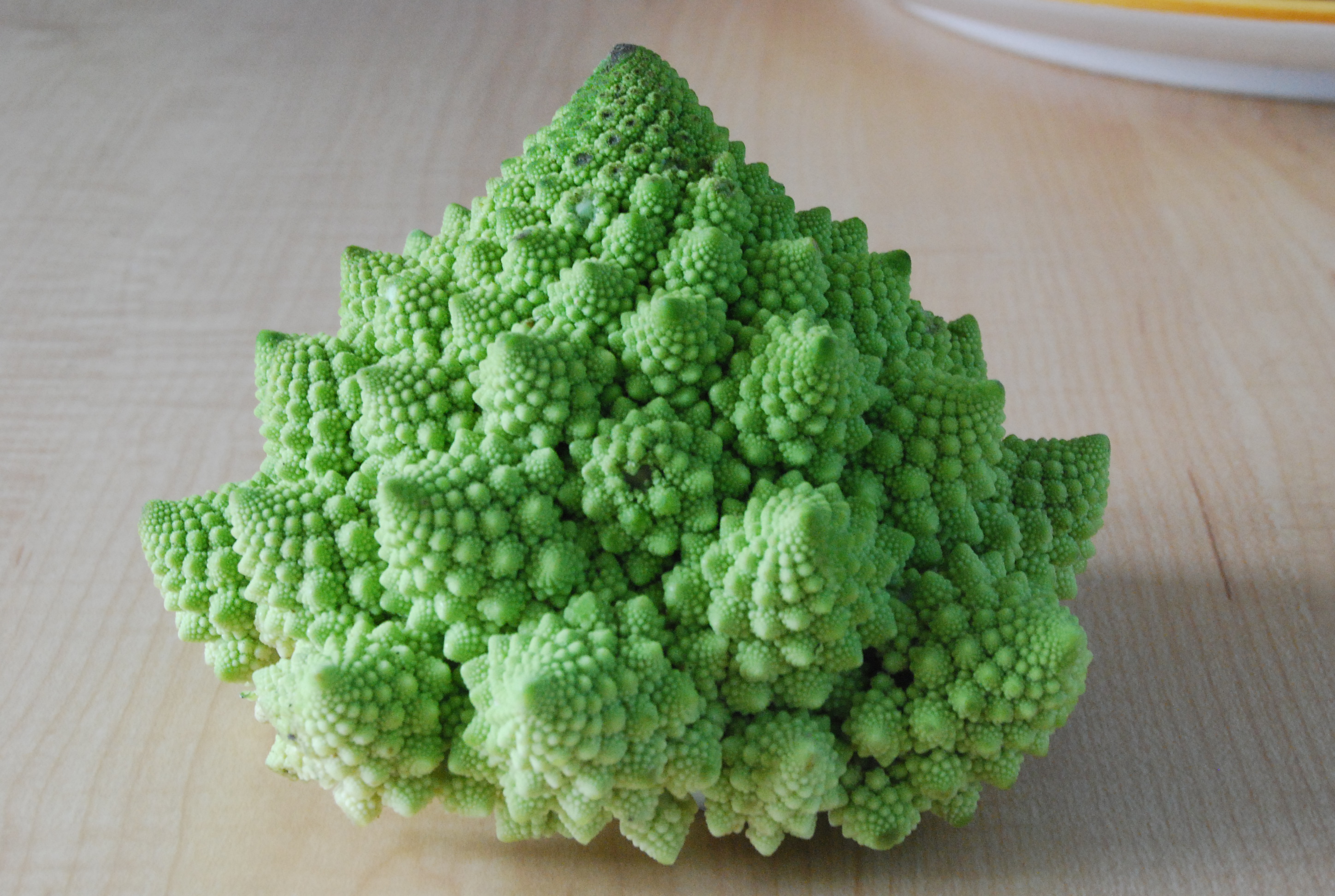
La palabra "patrón", por cierto, no implica la regularidad. Muchos patrones de conchas marinas son complejas e irregulares. Algunas conchas cono tienen lo que parecen ser colecciones al azar de los triángulos de diferentes tamaños, sin embargo, resulta que los patrones de este tipo son comunes en las ecuaciones semejantes a las de Turing. 
Brócoli Romanesco muestra fractales naturales. Wikimedia
De hecho, ellos son los fractales, un tipo complejo de la estructura geométrica puesto en conocimiento público por Benoît Mandelbrot en la década de 1970. Describió los fractales como "una forma geométrica áspera o fragmentada que puede dividirse en dos partes, cada una de ellas (al menos aproximadamente) una copia de tamaño reducido de la totalidad".

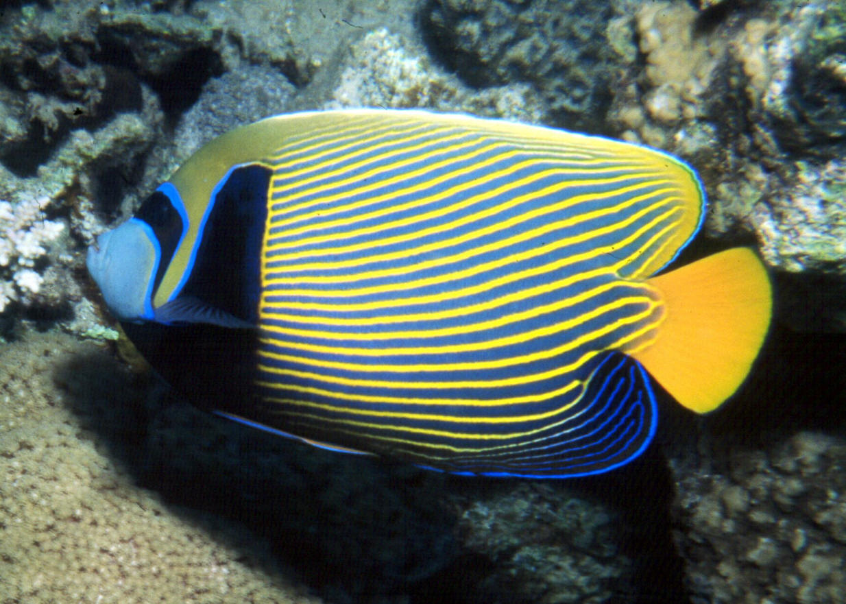
En 1995, los científicos japoneses Shigeru Kondo y Rihito Asai aplicaron las ecuaciones de Turing al hermoso pez ángel Pomacanthus Imperator tropical, que muestra sorprendentes rayas amarillas y púrpura. El modelo de Turing hizo una predicción sorprendente: las rayas del pez ángel se mueven a lo largo de su cuerpo (a diferencia de las de una cebra adulto, por ejemplo, que son fijos).

Pomacanthus imperator (Bloch 1787), pez Ángel Emperador(1). Distribuido ampliamente entre el Pacífico Central y del Sur hastalas costas del Océano Índico y el Mar Rojo. Longitud de unos 40cm. Adulto en el Mar Rojo. Imagen WetWebMedia
Parecía tremendamente poco probable, pero cuando Kondo y Asai fotografiaron ejemplares del pez ángel durante períodos de varios meses, encontraron que las rayas progresaban lentamente a través de su superficie. Por otra parte, los defectos en el patrón de rayas de otro modo regular, conocido como dislocaciones, se separaban y volvían a formarse exactamente como las ecuaciones de Turing lo predecían. Hacen esto porque las proteínas de pigmento se filtran de una célula a otra, dispersándose desde la cola del pez hacia su cabeza. (En los animales en los cuale las líneas son fijas, esto no sucede, pero una vez que el tamaño del animal y otros factores son conocidos, las matemáticas pueden predecir si sus marcas se desvían.)

Balones de fútbol portadores de enfermedades
La estructura de los virus - una causa importante de enfermedad en los seres humanos, animales y plantas - también puede explicarse por las matemáticas. Los virus son más grandes que la mayoría de las moléculas biológicas, pero podrían empaquetarse un millón de ellos en una sola bacteria. Superan en número a los seres humanos diez a la 25 a uno. Se conocen más de 5.000 tipos diferentes, y puede haber muchos millones más. Se componen de material genético envuelto en una capa de proteína, y cada virus tiene una estructura definida. La mayoría son icosaédrica o helicoidal: en forma de una pelota de fútbol o la forma de una escalera de caracol.

La comprensión de su estructura podría sugerir nuevas curas para la enfermedad. La herramienta matemática principal es la geometría, pero con una peculiaridad: se calcula en más de tres dimensiones.
La geometría clásica de Euclides se formula en dos dimensiones (el plano) o tres (el espacio). La forma de los virus nos conducen a algo menos conocido: la geometría de seis dimensiones. No estoy sugiriendo que los virus provienen de la sexta dimensión - que podría hacer un buen título para una película de ciencia-ficción, pero casi. Sin embargo, las matemáticas de las seis dimensiones resulta ser una buena manera de entender los virus en tres dimensiones, debido a las complicadas formas tridimensionales observadas en los virus que llegan a ser "sombras" o rebanadas más simples, de formas de seis dimensiones.

El punto culminante de texto geometría clásica de Euclides, los Elementos, identifica cinco sólidos regulares: cubo, tetraedro, el octaedro dodecaedro y el icosaedro. Los nombres, excepto el del cubo, se refieren al número de caras, cuatro, seis, ocho, doce y veinte, respectivamente. El cubo tiene caras cuadradas, el dodecaedro tiene los pentagonales, y los otros tres están hechos de triángulos equiláteros.

El elegante Icosaedro de Euclides, sin aplicación práctica por más de 2.000 años, resultó ser simplemente la forma correcta de hacer un virus. La gran pregunta era: ¿por qué?

Parte de la respuesta es la energía. Las cubiertas de los virus suelen ser construidas a partir de muchas copias de una única molécula de proteína, uno diferente para cada virus. Un conjunto de estas moléculas tiene la menor cantidad de energía - algo que la naturaleza encuentra conveniente - si está lo más cerca posible de ser una esfera.

Las cubiertas de los virus no pueden formar esferas exactas - tratar de encajar cien pelotas de tenis para hacer una esfera lisa - pero lo hacen lo mejor que pueden. Entre los sólidos de Euclides, el icosaedro es el más cercano a una esfera. Un icosaedro con sus esquinas cortadas es aún más esférico, debido a ésto, su uso para la mayoría de los balones utilizados en competiciones internacionales.

La cobertura proteínica de los virus icosaédricos están hecha de 20 triángulos y cada triángulo es un conjunto de unidades de proteínas, como las bolas al inicio de un juego de billar. En 1962 los biólogos Donald Caspar y Klug Aaron se dieron cuenta de que habían visto organizaciones como ésta, en el trabajo del arquitecto Buckminster Fuller.

Fuller es conocido por la "cúpula geodésica", un recinto más o menos esférico hizo mediante la instalación de un gran número de paneles triangulares entre sí (pensar en la cúpula del Proyecto Edén en Cornwall, aunque esto simplifica la estructura mediante el uso de hexágonos y pentágonos). Gaspar y Klug descubrieron que la mayoría de los virus tienen una geometría similar a las cúpulas de Fuller, que forman estructuras conocidas como pseudo-icosaedros - "pseudo" porque cada una de las 20 caras triangulares se subdivide en triángulos más.

Su geometría predice un número muy específico de las unidades de proteínas, tales como 32, 42, 72, 92, 162, 252 y 362, que forman las esquinas de la superficie. La teoría concuerda muy bien con virus reales - por ejemplo, la hepatitis infecciosa canina cuenta con 362 unidades, y el virus de la verruga humana tiene 72. En ambos casos, las unidades están dispuestos como una cúpula geodésica. Sin embargo, hay excepciones a la teoría de Caspar-Klug, tales como virus de simio 40, que puede causar tumores en los monos y los seres humanos.

Por poco más de diez años, el matemático de origen alemán Reidun Twarock estaba pensando este problema. Su respuesta fue desarrollar una teoría más general de la geometría de virus basada en las simetrías del icosaedro. A diferencia de la geometría de Euclides, sin embargo, utilizó formas de seis dimensiones, no tres.

Esto no es (del todo) tan complicado como parece, ya que "las dimensiones" en sentido amplio, significa "las variables en la ecuación". Imagine que el sistema solar: si desea trazar la posición de la tierra, lo que necesita saber dónde está en el espacio (tres dimensiones) y qué tan rápido se está moviendo a través del espacio (otros tres). Si luego quería representar la posición del sol, usted necesitaría otros seis. Para la luna, otros seis.

Como tal, las leyes matemáticas que gobiernan el movimiento se refieren a un espacio de 18 dimensiones. La configuración real de los cuerpos en cualquier instante se encuentra en común el espacio tridimensional, y es una especie de "sombra" de la descripción de 18 dimensiones.
Estamos muy acostumbrados a aplastar por las dimensiones de esta manera de tres a dos. Imagina que dibujas un árbol en el papel, por ejemplo. Pasar de seis o 18 dimensiones a tres utiliza la misma idea, sólo que con más variables.

Twarock usado esta idea para imaginar estructuras 3D virus como sombras de estructuras más simples en las dimensiones superiores. Por ejemplo, si la pila de un gran número de cubos juntos, como un tablero de ajedrez en 3D, y luego cortar a través de la pila de la manera correcta, se obtiene un patrón de mosaico elegante, con los dos triángulos y hexágonos (ver arriba). La pila original utiliza una sola forma, el cubo, pero hay dos formas aparecen en el corte.

O, para decirlo de otra manera, imagino mirando al gato, primero de frente, y luego de lado. En dos dimensiones, estas formas son muy diferentes. Pero mirar la vida, la respiración, el gato de tres dimensiones y las formas de sus diferentes partes tienen sentido.

Twarock utiliza un truco similar para las unidades de las proteínas de los virus icosaédrica. Un icosaedro es muy simétrica, en un sentido técnico - hay 120 maneras de girar o reflejar un icosaedro para que ocupe su espacio original. Si la disposición de las unidades proviene de un patrón en un espacio de dimensiones superiores, este nuevo modelo también debe tener la misma 120 simetrías. Hay una rama bien desarrollada de las matemáticas, la llamada teoría de grupos, que aborda este tipo de preguntas. Esto condujo a una lista específica de los patrones en un espacio de seis dimensiones.

La teoría resultante mejora en la de Gaspar y Klug. Es responsable de las estructuras excepcionales de virus del simio 40 y otros. Hay posibles implicaciones médicas, también. Una forma de ataque de un virus es interferir en su proceso de ensamblaje, y la geometría de los virus completamente ensamblado proporciona pistas sobre los posibles puntos débiles en este proceso.

Por otra parte, los virus icosaédricos a veces cambian los tubos de forma y la forma, que no son infecciosas. Un tratamiento que cambie la forma de icosaedro a tubo puede interferir con la replicación del virus y prevenir la enfermedad. Si los científicos pudieran "reprogramar" un virus para producir las unidades de la proteína que lo hizo tubular, pueden hacerlo inofensivo.

Paradoja del plancton
Nuestro último ejemplo proviene de las capas superiores de los océanos. Las aguas que rebosan de plancton, organismos que van desde criaturas microscópicas a las medusas pequeñas. Muchas son las larvas de adultos mucho más grandes. Todos ellos ocupan el mismo tipo de hábitat y compiten por mucho los mismos recursos.

Sin embargo, algo no está bien aquí. El principio de exclusión competitiva, introducido en 1932 por el biólogo ruso Georgii Gause, afirma que el número de especies en cualquier ambiente no debe ser mayor que el número disponible de "nichos", o formas de ganarse la vida. Si dos especies tratan de competir por el mismo nicho, la selección natural implica que uno de ellos debe ganar. Esta es la paradoja del plancton: los nichos son pocos, sin embargo, la diversidad es enorme - miles de especies.

La solución a la paradoja viene de la teoría del caos.
La dinámica clásica - basado en las leyes de Newton del movimiento - se centran en los estados estacionarios, donde nada cambia con el paso del tiempo, y periódicos de los Estados, en la misma secuencia de acontecimientos se repite una y otra vez. Una roca se encuentra en un estado de equilibrio si no se está moviendo y pasamos por alto la erosión. El ciclo de las estaciones es periódico, con un período de un año.

En la década de 1960, sin embargo, los matemáticos se dieron cuenta de que la visión convencional no había detectado otro tipo, más desconcertante de la conducta: el caos. Este es un comportamiento tan irregular que puede parecer aleatorio, pero no lo es.

Podría parecer que  tal comportamiento extravagante no tiene lugar en la naturaleza, pero el caos es completamente natural. Surge cada vez que la dinámica de un sistema combina todos sus componentes, hasta amasar mezclas de los ingredientes. Parece descabellado si usted está buscando soluciones que se pueden expresar por fórmulas limpias, ordenadas. Esas son raras, y la naturaleza no las necesita.

El modelo matemático que justifique principio de Gause asume las poblaciones no fluctúan con el tiempo. Pero esto toma el "equilibrio de la naturaleza" metáfora demasiado en serio. Los ecosistemas deben ser estables, pero un sistema estable, no necesita permanecer en el mismo estado para siempre, como una economía estable no es aquella en la que todo el mundo tiene exactamente la misma cantidad de dinero como lo hicieron ayer. Una población es estable si las fluctuaciones permanecen dentro de límites bastante estrechos. No es necesario que no haya fluctuaciones en absoluto.

La teoría del caos resuelve nuestro rompecabezas oceánico ya que permite a las fluctuaciones erráticas, pero pone límites a su tamaño. Fluctuaciones caóticas en las cuales diferentes especies utilizan los mismos recursos, pero en momentos diferentes. Incluso evitan la competencia directa, pero no lo hacen para que uno de ellos ganen y acaben con todos los demás. Lo hacen por turnos para acceder al mismo recurso. Así es como el caos resuelve la paradoja del plancton.

Vacas esféricas
Hay una vieja broma sobre un granjero que contrata a un grupo de matemáticos para ayudar a mejorar su producción de leche. Cuando se le presente con su informe, la primera frase dice: "Consideremos una vaca esférica". Esta historia expone un malentendido acerca de los modelos matemáticos. Ellos no tienen por qué ser una representación exacta de la realidad para ser útil. Una vaca esférica es inútil si usted desea dar a luz a un ternero, pero podría ser una aproximación razonable, si usted se está preguntando acerca de la propagación de una enfermedad de la piel.

Parte del arte de biomatemática es la selección de modelos de utilidad. Otra parte se está llevando a la biología en serio y no le falta algo crucial. Pero a veces también es necesario para probar una nueva idea en un entorno simplificado y ver dónde nos conduce.

Hay otra vieja broma, sobre un borracho buscando bajo una farola sus llaves."¿Le deje caer aquí?" "No, pero este es el único lugar donde no hay luz suficiente para ver." El contexto original, en la potencia y la razón humana por Joseph Weizenbaum, era una analogía con la ciencia, y el tema era exactamente lo contrario de la interpretación usual de la broma. En la ciencia, tienes que buscar en el poste de luz, o no vuelves a encontrar nada. Aun cuando las claves están en algún lugar a lo largo de la carretera en la cuneta, es posible encontrar una antorcha bajo el poste de luz. Ahora se puede buscar más lejos.

Me sorprendería si las matemáticas nunca llegaran a dominar el pensamiento biológico de la manera que lo hace la física, pero se está convirtiendo en una parte esencial de la disciplina: la biología del siglo 21 hace uso de las matemáticas de forma que nadie habría soñado en la inicio del 20. En el momento en que lleguemos a las matemáticas 22, y la biología hayan cambiado los demás más allá de todo reconocimiento, al igual que las matemáticas y la física hizo en los siglos 19 y 20. La ciencia está cambiando de una colección de pueblos a una comunidad en todo el mundo. Bienvenido al ecosistema global de la ciencia del mañana.

Ian Stewart es un profesor de matemáticas en la Universidad de Warwick y autor de "Matemáticas de la vida" (Profile Books, £ 20)